Calculate the Lm Curve. Again
We now need to present both stock (asset market) and flow (commodity market) equilibrium on the aforementioned graph. The conventional manner to do this is to put the real interest charge per unit on the vertical centrality and output (income and employment) on the horizontal ane. First, we nowadays again the equations of stock and menses equilibrium.
The weather condition of asset (stock) and goods market (flow) equilibrium as presented in the previous topic are, respectively
2. Y = ( a + δ + ΦBT + DSB)/(s + m) − μ/(s + one thousand) r + yard* /(due south + m) Y* − σ/(s + yard) Q
where we limited the domestic involvement rate simply as r without regard to the part of earth capital market place conditions in determining it---that will be incorporated subsequently. If you lot are not completely familiar with the derivation and meaning of these equations you should review the previous two topics again.
The combinations of r and Y for which Equation two holds can be presented equally a negative relationship between income and the real interest rate as shown in Figure ane. The downwardly sloping catamenia-equilibrium curve---normally non a direct line as here portrayed---is called the IS bend in textbooks and we will follow that naming convention here.
The label IS comes from the fact that in a airtight economy (one with no trade) the bend gives the combinations of income and the involvement charge per unit for which desired savings equals desired investment. In an open economy this curve gives the combinations of income and the interest rate for which the desired net capital outflow, represented by savings minus investment, equals the the desired electric current account balance---that is, for which South − I = BT + DSB. When there is no international merchandise, this condition becomes simply S − I = 0 .
A fall in the interest charge per unit leads to an expansion of investment, causing equilibrium output, income and emloyment to increase equally we move down along the IS bend. A autumn in the existent exchange rate shifts globe demand onto domestic goods, increasing income at each level of the existent involvement rate and shifting IS to the right. An increment in remainder-of-world income, or exogenous increase in consumption or investment or cyberspace exports at any given level of the real interest rate also causes the IS line to shift to the right and the equilibrium level of output, income and employment to increase.
To portray nugget equilibrium in terms of the relationship it implies between the real interest rate and the level of income, it is useful to rearrange Equation 1 to put r on the left side:
1a. r = − (1/θ) M/P + γ/θ − τ + (ε/θ) Y
Since ε/θ in this equation is preceded by a positive sign, the equation defines a positive human relationship between the real interest rate and level of income, belongings everything else abiding, and can be portrayed equally the upward sloping curve LM (portrayed every bit a straight line) in Figure 2. (The name LM, meaning liquidity-coin, is also traditional.) The LM curve gives the combinations of income and the interest charge per unit for which the demand for coin (or desired liquidity) equals the money supply and hence for which the domestic economy is in asset or stock equilibrium.
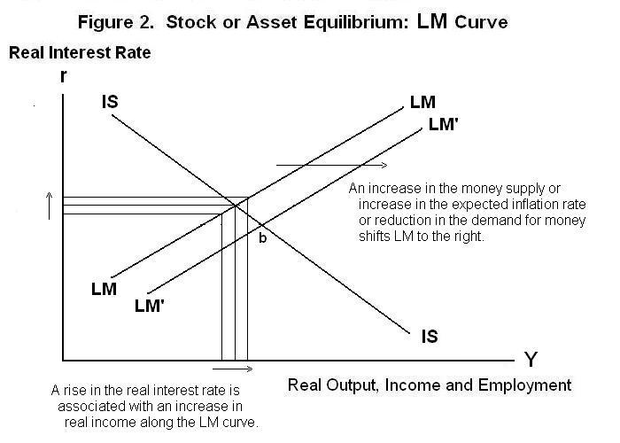
The intuition backside the positive slope of LM is as follows: An increment in the involvement rate reduces the need for money and an increment in income increases it. To keep the need for money equal to a constant money supply equally the involvement rate rises and we move along the LM curve, the level of income must increase.
An increase in the coin supply holding the real interest rate constant requires a higher level of income to make the demand for coin equal to that greater supply, shifting LM to the right. The combinations of income and the real involvement rate at which the demand for coin equals the supply now lie further to the right. An increase in the expected inflation rate at a given level of the real interest rate increases the cost of holding coin and reduces the quantity people chose to concur. This requires that the level of income rise at the given world real interest rate to bring desired money holdings back into line with the unchanged money supply and preserve asset equilibrium---the LM curve shifts to the right.
Overall equilibrium will occur where the IS and LM curves cross. In a an economy that is closed to international trade, an increase in the money supply in Figure two will shift LM to the correct causing the interest rate to fall as the public tries to reestablish portfolio equilibrium by purchasing assets. The fall in the interest rate volition cause output, income and employment to increase. The involvement rate volition fall and income will increment until the quantity of money demanded has increased by an amount equal to the increase in the coin supply. The new equilibrium volition exist at indicateb in Figure ii.
Total portrayal of equilibrium also requires that nosotros add a vertical line YF to portray the full-employment level of income which the equilibrating process will eventually attain in the long-run. This is shown in Figure three.
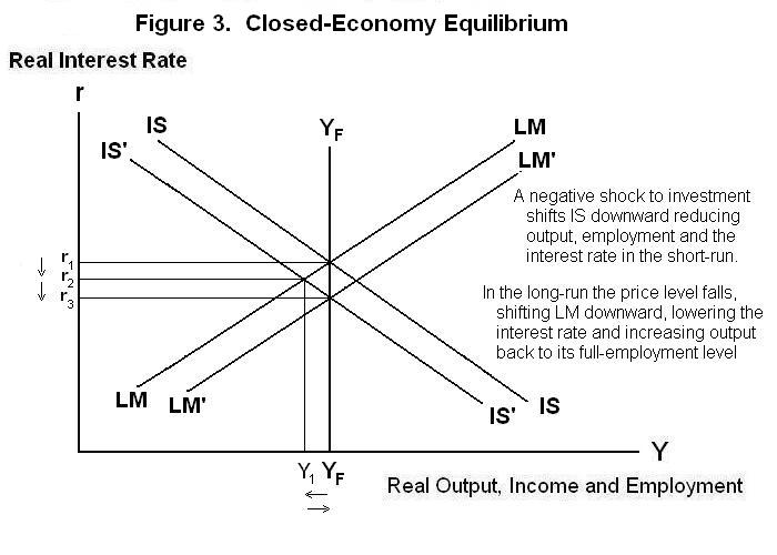
Starting with a full-employment situation where IS and LM cross, allow the states assume that at that place is a decline in desired investment so that the IS curve shifts downwardly to IS'. In the short run before the price level tin adjust the existent interest rate will fall from r1 to r2 and output and income autumn from their full-employment levels to Y1 . As time passes the toll level will fall, increasing the real money stock and shifting the LM bend down to LM'. As a result, the existent involvement rate will fall from rtwo to r3 and income and employment volition render to their full-employment levels.
The above analysis assumes, unrealistically, that our economy is closed to international trade and capital movements. When we incorporate these elements an boosted line has to exist added to the graph---the horizontal rZ line in Figure 4.
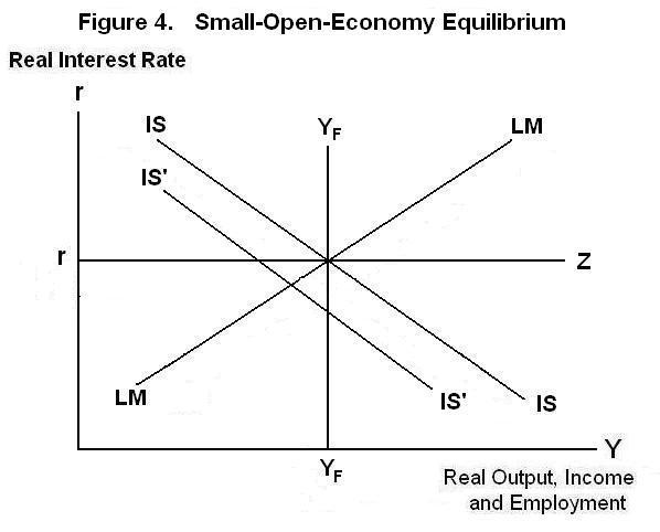
The rZ line imposes on our modest open economy the effect of world market conditions on the determination of the domestic real involvement rate. Since domestic assets are endemic earth-wide and the domestic economy is small, the interest rate on those assets will exist determined by the willingness of world residents to hold them. The domestic real interest rate volition thus equal the foreign real interest rate plus a premium that reflects the take chances of holding domestic assets rather than rest-or-globe avails. The domestic involvement rate will also differ from the foreign interest charge per unit by an amount to compensate for whatever expected uppercase gain or loss on domestic assets resulting from expected future changes in the domestic real exchange charge per unit.
Overall total-employment equilibrium of the small open economy will occur, of class, where the IS and LM curves cross at the signal at which the vertical YF line and the horizontal rZ as well cross. Simply suppose now that the IS bend shifts down to IS'. Given the fact that the domestic interest charge per unit cannot change, how will a new equilibrium be established in the brusk and long runs? The next two topics will develop the answer to this question. First, notwithstanding, information technology is time for a test. As e'er think upwardly your ain answers to the questions before looking at the answers provided.
Question 1
Question 2
Question 3
Source: https://www.economics.utoronto.ca/jfloyd/modules/islm.html
0 Response to "Calculate the Lm Curve. Again"
Post a Comment